Comparing multivariate data
Symmetric methods for comparing two matrices
Jes & Priscilla
Assigned Reading:
Sections 10.5 (p. 597) and 11.5 (p. 696) from: Legendre, P. and L. Legendre. 2012. Numerical Ecology. Elsevier. link
Skim the math to whatever degree you desire.
Key Points
Use a symmetric methods when you don’t have a hypothesis about the direction of effects between two matrices.
Examples? Counter-examples?
Compare similarity/distance matrices
“These methods should not be used to test hypotheses about relationships between the original data tables.”
- Use Chapter 7 to choose an appropriate distance measure for your data.
Mantel test
- Box 10.2 on p. 600
- Tests whether distances among objects are monotonically related to one another.
- Steps:
- Compute a Mantel statistic that is the scalar product of the (non-diagonal) values in (half of) the two distance matrices. (See Figure 10.19 on p. 599)
- \(z_M\) : raw distances
- \(r_M\) : use standardized distances and divide by \(n(n-1)/2 - 1\) to get value between -1 and 1.
- Test whether \(z_M\) is significantly larger than expected by permuting the objects in one of the original data matrices used to compute one of the distance matrices. The generates a distribution of potential \(z_M\) values under the null hypothesis.
- Compute a Mantel statistic that is the scalar product of the (non-diagonal) values in (half of) the two distance matrices. (See Figure 10.19 on p. 599)
- Use Spearman (rank-based) correlation coefficient is non-linearity expected.
- Distance matrices must be derived independently from one another on the same set of objects.
- Many applications of Mantel test probably should be done using canonical analysis(e.g. distribution of organisms with respect to environment controlling for distance among sites)
- Do not use Mantel test to make conclusions about correlations in the original data.
Analysis of Similarity (ANOSIM) and PERMANOVA
- ANOSIM tests whether distances between groups are greater than within groups.
- PERMANOVA tests whether distance differ between groups. This wasn’t in the original reading for class, but you can find the method in Anderson (2001).
- Both tests are sensitive to unbalanced designs and differences in dispersion (variance) within groups (e.g. not good when your groups have different variability). Anderson and Walsh (2013) conducted a simulation-based comparison of PERMANOVA and ANOSIM and found that PERMANOVA is more robust in general for ecological data, but still sensitive to heterogeneity of variance among groups. You should evaluate this assumption before using either test.
- ANOSIM Steps:
- Rank distances within the distance matrix, then compute the statistic \(R = \frac{mean(rank_{between}) - mean(rank_{within})}{n(n-1)/4}\).
- Test whether \(R\) is larger than expected by permuting original objects.
- PERMANOVA Steps:
- Calculate an F ratio comparing \(F \sim \frac{SS_{within groups}}{SS_across groups}\), where \(SS\) means adding up the sum of the squares of the distances.
- Test whether \(F\) is smaller than expected by chance by permuting the original objects.
- Groups should be defined a priori and not derived from distances.
Compare two data tables
- Methods often used to jointly analyze variation two communities at the same set of sites.
- Do not use to compare matrices that measure the same variables (e.g. before-after studies or control-impact experiments) because the analysis does not know that the variables are the same. (Use RDA or PCA instead.)
- Both co-inertia and procrustes analyses can handle more variables than observations (e.g. more species than sites) as well as collinearity among variables.
- Canonical correlation analysis (CCorA) is generally not recommended because it assumes multivariate normality of quantitative variables.
Co-inertia analysis
- Creates an ordination based on two covariance between two data matrices and plots both matrices in the same ordination space along with their variables.
- Steps:
- Calculate cross-covariance matrix between variables in two matrices.
- Calculate eigenvalues and eigenvectors of covariance matrix. Eigenvectors give the axes of the ordination.
- Project the two matrices in the ordination space and use arrows to connect the two points measured on the same object.
- Add arrows for each of the variables in the two matrices.
- The total co-inertia is the sum of the squared covariances and the eigenvalues partition this among ordination axes.
- Co-inertia analysis will preserve Euclidean or Mahalanois distances between objects depending on how projected matrices are scaled.
- Can use data transformations prior to analysis (recommended for species occurrence data).
- If so, do a principal coordinate analysis on the two distance martices and use the axes corresponding to positive eigenvalues as the data tables input into co-inertia analysis.
- \(RV\) coefficient is a statistic that measures correlation of two data matrices whose significance is tested by permutation.
Procrustes analysis
- Creates a “compromise” ordination of two matrices measured on the same objects in order to visualize differences between two martices.
- Algorithm rotates the matrices to minimize the sum of squared distances between corresponding objects.
- Very similar to co-inertia analysis, but uses different matrices for plotting.
- PROTEST method: compute symmetric orthogonal Procrustes statistic \(m^2\) to measure similarity between two data matrices.
Multiple factor analysis
- Used to compare sets of variables- all variables within a set must be the same type.
- Compute PCA on each variable set separately, then compute PCA of concatenated PC axes from all sets (that are first multiplied by a number to give equal weight to each set).
- Project variable sets onto ordination plot to compare their correlation.
R packages and functions
vegan: functions for community composition analysis
mantel()protest()anosim()adonis()for PERMANOVAbetadisper()for testing homogeneity of within-group variances
ecodist: functions for analysis of ecological dissimilarity
mantel()MRM()
ape: functions fo phylogenetic analysis
mantel.test()
ade4: functions for multivariate analysis for ecologists
mantel.rtest()coinertia()on two separate ordinations produced bydudi.pca()ordudi.pco()mfa()on aktabdataframe that divides variables into “blocks” produced byktab.data.frame()
Analysis Example
Matrix comparisons
The following tests are used to test relationships between association matrices (i.e. distance or similarity matrices) not raw data! + Mantel test + Partial Mantel test + Multiple regression on distance matrices
# Load packages
library(readr)
library(dplyr)
library(phyloseq)
library(vegan)
library(ade4)
library(ggplot2)
Mantel test
Compare two distance/similarity matrices that were obtained independently of each other
# Transpose otu tables from both phyloseqs and convert to data frame
data_16s <- as.data.frame(t(otu_table(merged_16s)))
data_CO1 <- as.data.frame(t(otu_table(merged_CO1)))

# Calculate distance using Bray-Curtis
DM16s <- distance(merged_16s,"bray")
DMco1 <- distance(merged_CO1, "bray")

# Mantel test (using three different methods)
mantel(DMco1, DM16s, method = "pearson", permutations = 999)
##
## Mantel statistic based on Pearson's product-moment correlation
##
## Call:
## mantel(xdis = DMco1, ydis = DM16s, method = "pearson", permutations = 999)
##
## Mantel statistic r: 0.1919
## Significance: 0.004
##
## Upper quantiles of permutations (null model):
## 90% 95% 97.5% 99%
## 0.0508 0.0797 0.0999 0.1480
## Permutation: free
## Number of permutations: 999mantel(DMco1, DM16s, method = "spearman", permutations = 999) ##
## Mantel statistic based on Spearman's rank correlation rho
##
## Call:
## mantel(xdis = DMco1, ydis = DM16s, method = "spearman", permutations = 999)
##
## Mantel statistic r: 0.1369
## Significance: 0.003
##
## Upper quantiles of permutations (null model):
## 90% 95% 97.5% 99%
## 0.0700 0.0897 0.1065 0.1190
## Permutation: free
## Number of permutations: 999mantel(DMco1, DM16s, method = "kendall", permutations = 999)##
## Mantel statistic based on Kendall's rank correlation tau
##
## Call:
## mantel(xdis = DMco1, ydis = DM16s, method = "kendall", permutations = 999)
##
## Mantel statistic r: 0.1113
## Significance: 0.012
##
## Upper quantiles of permutations (null model):
## 90% 95% 97.5% 99%
## 0.0642 0.0813 0.0915 0.1148
## Permutation: free
## Number of permutations: 999# Plot the distances against each other (just to see)
plot(DMco1, DM16s, type = "p")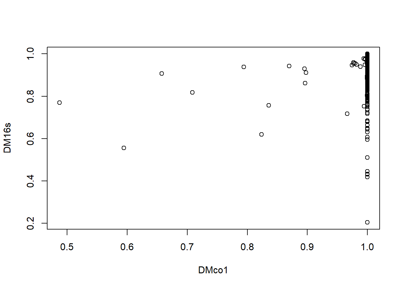
Canonical Analysis
- Used to analyze relationships between two rectangular data tables
The following tests can use raw data, not distance matrices (e.g. two community composition matrices)
- Co-interia analysis
- RV coefficient
- Procrustes
Co-inertia analysis
- Search for common structures between two data sets describing the same objects by projecting them onto a common multivariate space
- Uses two responses containing different variables
dudi.16s <- dudi.pca(data_16s, scale=T, scan=F, nf=5)
dudi.c01 <- dudi.pca(data_CO1, scale=T, scan=F, nf=5)
co.in.data <- coinertia(dudi.16s, dudi.c01, scan=F, nf=5)
summary(co.in.data)
## Coinertia analysis
##
## Class: coinertia dudi
## Call: coinertia(dudiX = dudi.16s, dudiY = dudi.c01, scannf = F, nf = 5)
##
## Total inertia: 5763
##
## Eigenvalues:
## Ax1 Ax2 Ax3 Ax4 Ax5
## 665.7 547.4 513.0 420.8 379.7
##
## Projected inertia (%):
## Ax1 Ax2 Ax3 Ax4 Ax5
## 11.550 9.498 8.901 7.301 6.588
##
## Cumulative projected inertia (%):
## Ax1 Ax1:2 Ax1:3 Ax1:4 Ax1:5
## 11.55 21.05 29.95 37.25 43.84
##
## (Only 5 dimensions (out of 36) are shown)
##
## Eigenvalues decomposition:
## eig covar sdX sdY corr
## 1 665.6710 25.80060 6.254968 4.257402 0.9688579
## 2 547.4037 23.39666 9.136070 2.684524 0.9539535
## 3 512.9977 22.64945 8.737747 2.794415 0.9276142
## 4 420.8116 20.51369 7.022618 4.022149 0.7262508
## 5 379.6807 19.48540 7.333985 3.131459 0.8484427
##
## Inertia & coinertia X (dudi.16s):
## inertia max ratio
## 1 39.12463 118.1844 0.3310474
## 12 122.59240 222.3012 0.5514699
## 123 198.94062 311.9950 0.6376404
## 1234 248.25778 387.0472 0.6414147
## 12345 302.04511 455.8617 0.6625805
##
## Inertia & coinertia Y (dudi.c01):
## inertia max ratio
## 1 18.12547 21.19416 0.8552106
## 12 25.33214 39.64262 0.6390127
## 123 33.14089 48.89262 0.6778301
## 1234 49.31858 58.03207 0.8498505
## 12345 59.12461 66.77656 0.8854097
##
## RV:
## 0.518941randtest(co.in.data, nrepet = 999)## Monte-Carlo test
## Call: randtest.coinertia(xtest = co.in.data, nrepet = 999)
##
## Observation: 0.518941
##
## Based on 999 replicates
## Simulated p-value: 0.927
## Alternative hypothesis: greater
##
## Std.Obs Expectation Variance
## -1.342338615 0.601967484 0.003825686plot(co.in.data)
RV coefficient
- multivariate generalization of Pearson correlation coefficient
- tests whether two matrices are linked
- value is given through co-inertia analysis but can also try
RV.rtest(data_16s, data_CO1)
Procrustes
- measure of concordance, similarity, between two data matrices
- more powerful than Mantel test
# Only run this once and then re-load
#procrust.data <- protest(data_CO1, data_16s)

# Save and reload the Procrustes analysis results
#save(procrust.data, file = "data/psanjuan/procrust_data.RData")
load("data/psanjuan/procrust_data.RData")

summary(procrust.data)plot(procrust.data)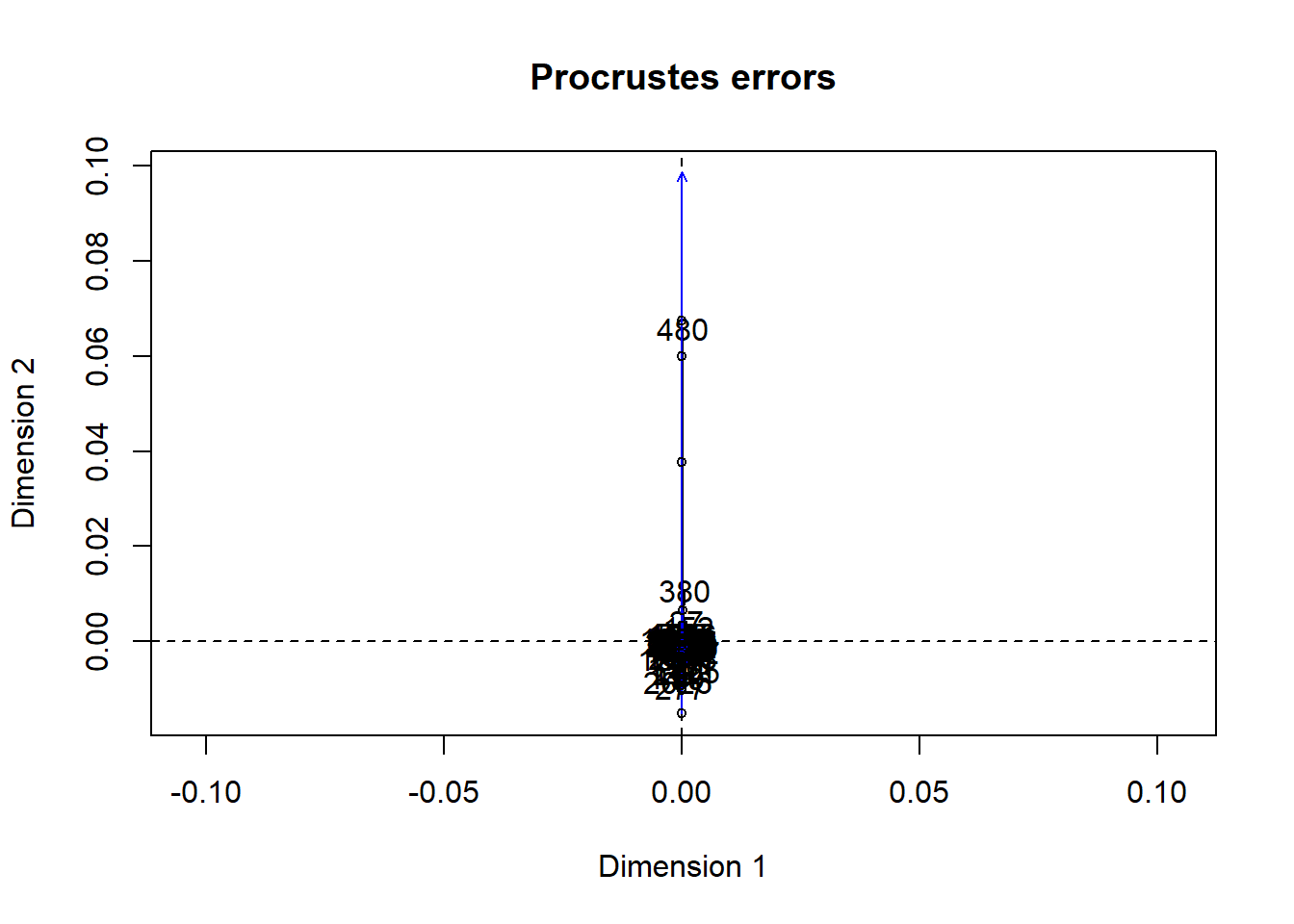
Discussion Questions
- What are some examples of datasets that are compatible for these tests? Any rule of thumb to easily identify an appropriate test (beside trying all of them)?
- Any experience with this type of analyses?
- “Which method should be used for symmetric analysis of two data sets?”
Further Readings
For information on three-table methods see:
- Dray, S. P. et al. 2014. Combining the fourth-corner and RLQ methods for assessing trait responses to environmental variation. Ecology 95: 14-21. DOI: 10.1890/13-0196.1. and Supplement 1: A tutorial to perform fourth-corner and RLQ analyses in R. Ecological Archives E095-002-S1