GLM with zero-inflated data
Tad; Nick Hendershot
Assigned Reading:
Chapter 11 from: Zuur, A. F., Ieno, E. N., Walker, N., Saveliev, A. A. and Smith, G. M. 2009. Mixed Effects Models and Extensions in Ecology with R. Springer. link
Key Points
Definition and why it is a problem
When the number of zeros is so large that the data do not readily fit standard distributions (e.g. normal, Poisson, binomial, negative-binomial and beta), the data set is referred to as zero inflated (Heilbron 1994; Tu 2002).
The source of the zeroes matters: Non-detection (false zeros) or true zeroes?
A special case: zero-truncated count data
e.g., Number of days that road-kills remain on the road
Poisson and NB models can be adjusted to exclude the probability that yi = 0 (equation 11.8 on p. 265).
family = pospoissonandfamily = posnegbinomialin VGAM package
More often, we get too many zeros (zero-inflated)
How to detect zero-inflation: Frequency plot to know how many zeroes we would expect
Zero-inflation can cause overdispersion (but accounting for zero-inflation does not necessarily remove overdispersion).
Two-part and mixture models for zero-inflated data (Table 11.1).
Fundamental difference: In two-part models, the count process cannot produce zeros (the distribution is zero-truncated). In mixture models, it can.
In other words, two-part models do not distinguish true and false zeros (Fig 11.4), whereas mixture models do, at least statistically (Fig 11.5).
Two-part models
Source of zeroes is NOT considered
First step: zero or nonzero? Binomial model used to model probability of zeroes
Second step: zero-truncated model used to model the count data
Can do this separately (two models) or combine to use one model (
hurdle()in pscl package)
Mixture models
Zeroes are modeled explicitly as coming from multiple processes: true zeroes and false zeroes are modeled as being generated from different processes
zeroinfl()in pscl package
Steps
Choose model type
Prune variables (
drop1())Model validation (extract residuals and plot vs. all predictors or measured variables)
Model interpretation
But how to choose model type?
- Options: common sense, model validation, information criteria, hypothesis tests (Poisson or NB), comparison of observed and fitted values
Analysis Example
# Read in OBFL data

OBFL <- read.csv('./data/OBFL.csv',
                 header = T)

############################################################
library(lattice)
library(MASS)
require(pscl) # alternatively can use package ZIM for zero-inflated models
library(lmtest)
Data includes counts of ochre-bellied flycatcher (OBFL) captures across deforestation and agricultural intensification gradient in southern Costa Rica. Specifically, sampling date, Counts (number of captures at site on a given day), Site Code and standardized mean canopy cover at the site (Canopy.std).
Here we will be looking at the relationship between number of captured individuals and canopy cover using a series of GLMs to deal with overdispersion. In reality we could use a GLMM with this data, but we will stick with GLMs for simplicity.
The steps and code use for these anlyses pull from heavily from:
1. Zuur, A. F., Ieno, E. N., Walker, N., Saveliev, A. A. and Smith, G. M. 2009. Mixed Effects Models and Extensions in Ecology with R.
2. Zuur, A. F. and Ieno, E. N. 2016. Beginner’s Guide to Zero-Inflated Models with R.
Relationship between Counts and Canopy Cover
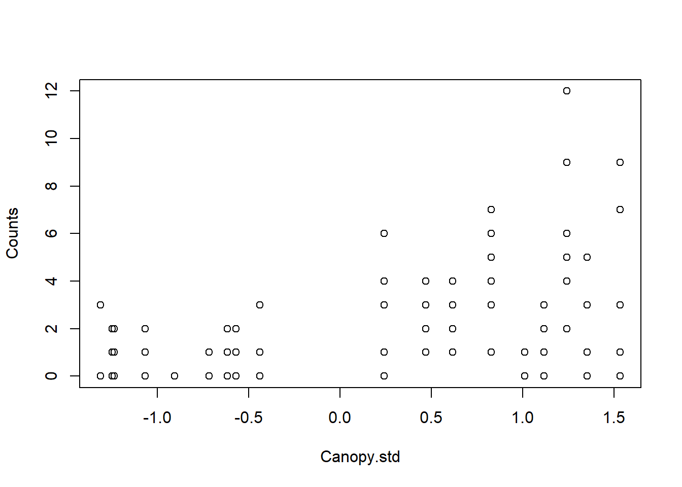
Let’s do a quick check for Zero-Inflation in the data
100*sum(OBFL$Counts == 0)/nrow(OBFL)## [1] 40.36697That’s pretty high! ~ 40% of our data are zeros
While our data seems to be zero-inflated, this doesn’t necessarily mean we need to use a zero-inflated model. In many cases, the covariates may predict the zeros under a Poisson or Negative Binomial model. So let’s start with the simplest model, a Poisson GLM.
Poisson GLM
\(Counts_i \sim Poisson(\mu_i)\)
\(E(Counts_i) = \mu_i\)
\(var(Counts_i) = \mu_i\)
\(log(\mu_i) = \alpha + \beta_1 * Canopy.std_i\)
## Poisson GLM
M1 <- glm(Counts ~ Canopy.std,
          family = 'poisson',
          data = OBFL)

summary(M1)
##
## Call:
## glm(formula = Counts ~ Canopy.std, family = "poisson", data = OBFL)
##
## Deviance Residuals:
## Min 1Q Median 3Q Max
## -2.8609 -1.1927 -0.9465 0.6633 3.7112
##
## Coefficients:
## Estimate Std. Error z value Pr(>|z|)
## (Intercept) 0.21602 0.09701 2.227 0.026 *
## Canopy.std 0.77757 0.08953 8.685 <2e-16 ***
## ---
## Signif. codes: 0 '***' 0.001 '**' 0.01 '*' 0.05 '.' 0.1 ' ' 1
##
## (Dispersion parameter for poisson family taken to be 1)
##
## Null deviance: 286.66 on 108 degrees of freedom
## Residual deviance: 195.32 on 107 degrees of freedom
## AIC: 373.4
##
## Number of Fisher Scoring iterations: 5## Check for over/underdispersion in the model
E2 <- resid(M1, type = "pearson")
N <- nrow(OBFL)
p <- length(coef(M1))
sum(E2^2) / (N - p)## [1] 1.809869Looks like our model produces overdisperion. There are many reasons why this might be the case, but for now we are going to try to use a negative binomial GLM using the ‘glm.nb’ function in the ‘MASS’ package
Negative Binomial GLM
\(Counts_i \sim NB(\mu_i, theta)\)
\(E(Counts_i) = \mu_i\)
\(var(Counts_i) = (\mu_i + \mu_i^{2})/theta\)
\(log(\mu_i) = \alpha + \beta_1 * Canopy.std_i\)
M2 <- glm.nb(Counts ~ Canopy.std,
             data = OBFL)

summary(M2)
##
## Call:
## glm.nb(formula = Counts ~ Canopy.std, data = OBFL, init.theta = 1.864363167,
## link = log)
##
## Deviance Residuals:
## Min 1Q Median 3Q Max
## -2.1169 -1.0006 -0.7327 0.4588 2.1316
##
## Coefficients:
## Estimate Std. Error z value Pr(>|z|)
## (Intercept) 0.1952 0.1223 1.597 0.11
## Canopy.std 0.8290 0.1194 6.945 3.78e-12 ***
## ---
## Signif. codes: 0 '***' 0.001 '**' 0.01 '*' 0.05 '.' 0.1 ' ' 1
##
## (Dispersion parameter for Negative Binomial(1.8644) family taken to be 1)
##
## Null deviance: 162.32 on 108 degrees of freedom
## Residual deviance: 109.99 on 107 degrees of freedom
## AIC: 346.13
##
## Number of Fisher Scoring iterations: 1
##
##
## Theta: 1.864
## Std. Err.: 0.610
##
## 2 x log-likelihood: -340.135# Dispersion statistic
E2 <- resid(M2, type = "pearson")
N <- nrow(OBFL)
p <- length(coef(M2)) + 1 # '+1' is for variance parameter in NB
sum(E2^2) / (N - p)## [1] 0.9773875Looks like the Negative Binomial GLM resulted in some minor underdispersion. In some cases, this might be OK. But in reality, we want to avoid both under- and overdispersion.
Overdispersion can bias parameter estimates and produce false significant relationships. On the otherhand, underdisperion can mask truly significant relationships. So let’s try to avoid all of this.
Zero-Inflated Poisson GLM
\(Counts_i \sim ZIP(\mu_i, \pi_i)\)
\(E(Counts_i) = \mu_i * (1-\pi_i)\)
\(var(Counts_i) = (1-\pi_i) * (\mu_i + \pi_i * \mu_i^{2})\)
\(log(\mu_i) = \beta_1 + \beta_2 * Canopy.std\)
\(log(\pi_i) = \gamma_1 + \gamma_2 * Canopy.std\)
In zero-inflated models, it is possible to choose different predictors for the counts and for the zero-inflation. You might expect different variables to be driving presence/absence vs. total number of individuals. We will keep it simple and use the same covariate in both parts.
M3 <- zeroinfl(Counts ~ Canopy.std | ## Predictor for the Poisson process
                 Canopy.std, ## Predictor for the Bernoulli process;
               dist = 'poisson',
               data = OBFL)

summary(M3)
##
## Call:
## zeroinfl(formula = Counts ~ Canopy.std | Canopy.std, data = OBFL,
## dist = "poisson")
##
## Pearson residuals:
## Min 1Q Median 3Q Max
## -1.7794 -0.6838 -0.4998 0.6525 4.1540
##
## Count model coefficients (poisson with log link):
## Estimate Std. Error z value Pr(>|z|)
## (Intercept) 0.5515 0.1440 3.830 0.000128 ***
## Canopy.std 0.5951 0.1443 4.123 3.73e-05 ***
##
## Zero-inflation model coefficients (binomial with logit link):
## Estimate Std. Error z value Pr(>|z|)
## (Intercept) -1.1273 0.3643 -3.094 0.00197 **
## Canopy.std -1.0102 0.4406 -2.293 0.02185 *
## ---
## Signif. codes: 0 '***' 0.001 '**' 0.01 '*' 0.05 '.' 0.1 ' ' 1
##
## Number of iterations in BFGS optimization: 11
## Log-likelihood: -177.1 on 4 Df# Dispersion statistic
E2 <- resid(M3, type = "pearson")
N <- nrow(OBFL)
p <- length(coef(M3))
sum(E2^2) / (N - p)## [1] 1.368017Still a some overdispersion in the ZIP. Let’s try a ZINB
Zero-Inflated Negative Binomial GLM
\(Counts_i \sim ZINB(\mu_i, \pi_i)\) Not actually sure how to formulate this part for ZINB??
\(E(Counts_i) = \mu_i * (1-\pi_i)\)
\(var(Counts_i) = (1-\pi_i) * (\mu_i + \pi_i^{2}/k) + \mu_i^{2} * (\pi_i^{2} + \pi_i)\)
\(log(\mu_i) = \beta_1 + \beta_2 * Canopy.std\)
\(log(\pi_i) = \gamma_1 + \gamma_2 * Canopy.std\)
M4 <- zeroinfl(Counts ~ Canopy.std |
                 Canopy.std,
               dist = 'negbin',
               data = OBFL)
summary(M4)
##
## Call:
## zeroinfl(formula = Counts ~ Canopy.std | Canopy.std, data = OBFL,
## dist = "negbin")
##
## Pearson residuals:
## Min 1Q Median 3Q Max
## -1.1964 -0.6732 -0.4155 0.5077 3.9661
##
## Count model coefficients (negbin with log link):
## Estimate Std. Error z value Pr(>|z|)
## (Intercept) 0.4323 0.1737 2.489 0.01280 *
## Canopy.std 0.5892 0.1710 3.446 0.00057 ***
## Log(theta) 0.8332 0.3672 2.269 0.02326 *
##
## Zero-inflation model coefficients (binomial with logit link):
## Estimate Std. Error z value Pr(>|z|)
## (Intercept) -3.082 1.481 -2.081 0.0374 *
## Canopy.std -2.725 1.238 -2.201 0.0278 *
## ---
## Signif. codes: 0 '***' 0.001 '**' 0.01 '*' 0.05 '.' 0.1 ' ' 1
##
## Theta = 2.3008
## Number of iterations in BFGS optimization: 18
## Log-likelihood: -168.4 on 5 Df# Dispersion Statistic
E2 <- resid(M4, type = "pearson")
N <- nrow(OBFL)
p <- length(coef(M4)) + 1 # '+1' is due to theta
sum(E2^2) / (N - p)## [1] 0.992081This is really close to 1, which looks great.
We can compare the two zero-inflated models using the Likelihood ratio test
lrtest(M3, M4)## Likelihood ratio test
##
## Model 1: Counts ~ Canopy.std | Canopy.std
## Model 2: Counts ~ Canopy.std | Canopy.std
## #Df LogLik Df Chisq Pr(>Chisq)
## 1 4 -177.14
## 2 5 -168.37 1 17.538 2.816e-05 ***
## ---
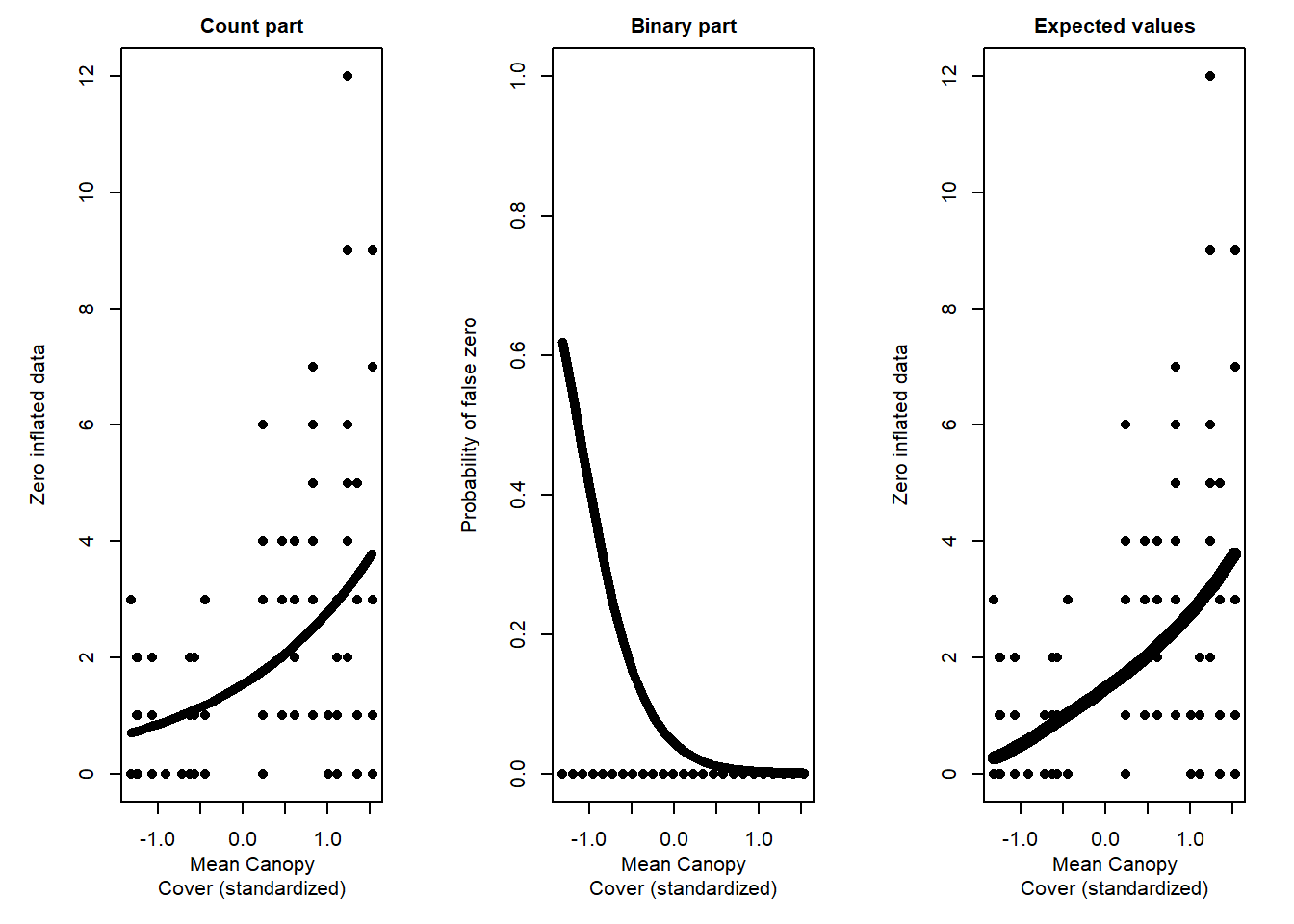
## Signif. codes: 0 '***' 0.001 '**' 0.01 '*' 0.05 '.' 0.1 ' ' 1Results show that the second model- the ZINB- is the best choice. So let’s stick with this model and plot the results
Sketch fitted and predicted values
Discussion Questions
- When might you add differet covariates into the Bernoulli vs Poisson/NB portion of Zero-inflated models?
- How close to 1 do dispersion statistics need to be?
- Anyone have experience with the two-step Zero-Altered models?