GLM with count, binary, and proportional data

Key Points

Analysis Example

GLM for Presence/Absence Data

Students in the course can download the data from our Canvas site into a data folder in their working directory.

First, I’ll read in the data:

# Read in my data from data folder in your working directory
aedes_dat <- read.csv("data/AedesData_EcoStats_Example.csv") 

attach(aedes_dat)

Next, I want to do some quick data exploration:

hist(Proportion, breaks=16, xlab = "aedes proportion", freq = FALSE)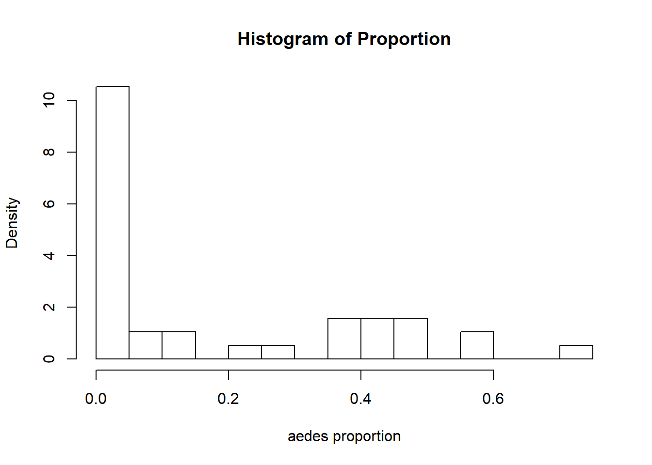

hist(aedes, breaks=16, xlab = "vegetation cover", freq = FALSE)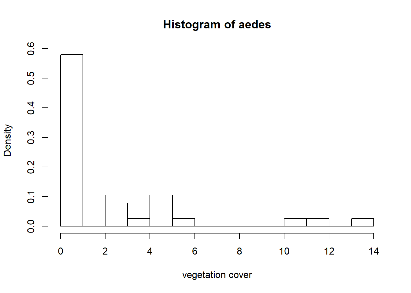

dotchart(aedes, xlab = "Aedes count",
         ylab = "Order of data", labels = F)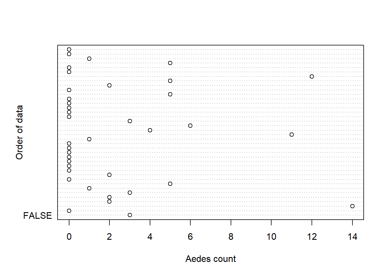

dotchart(Proportion, xlab = "Proportion Aedes",
         ylab = "Order of data", labels = F)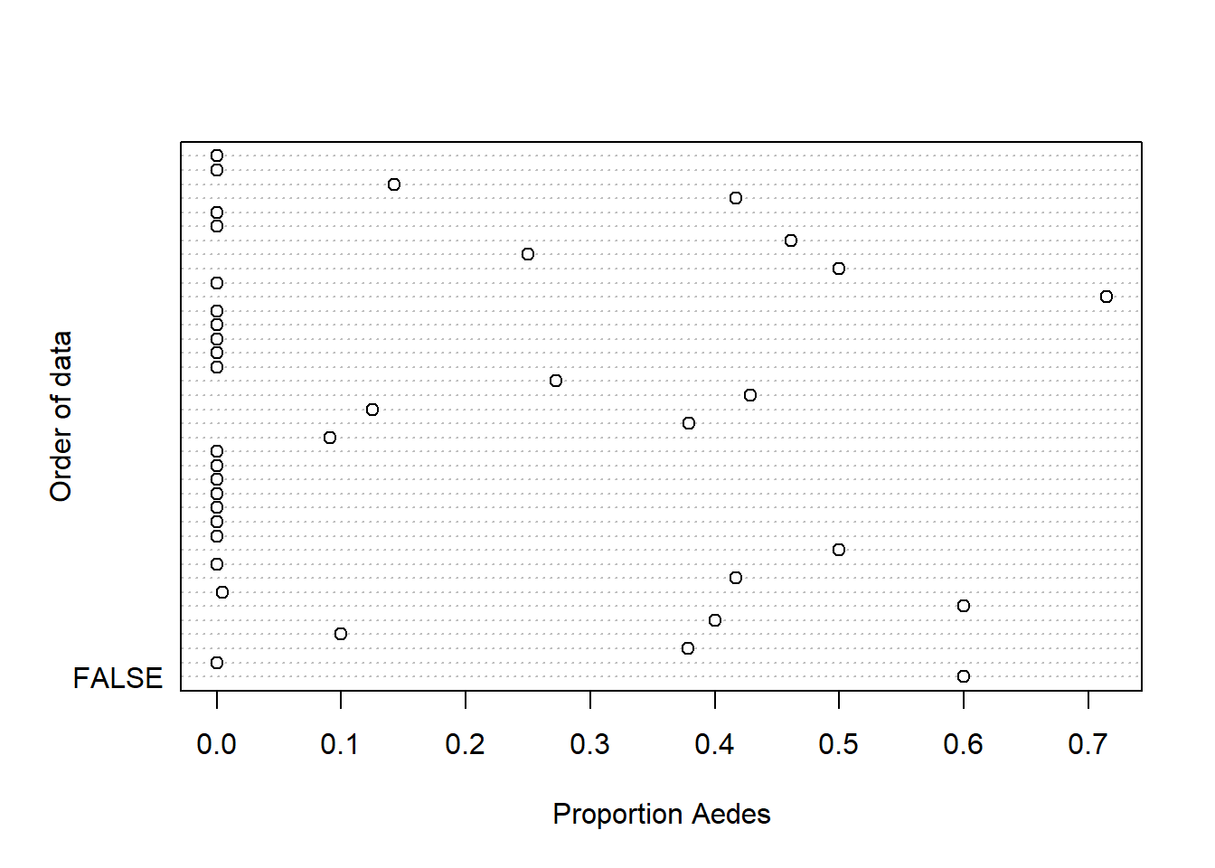

plot(Vegetation,Presence)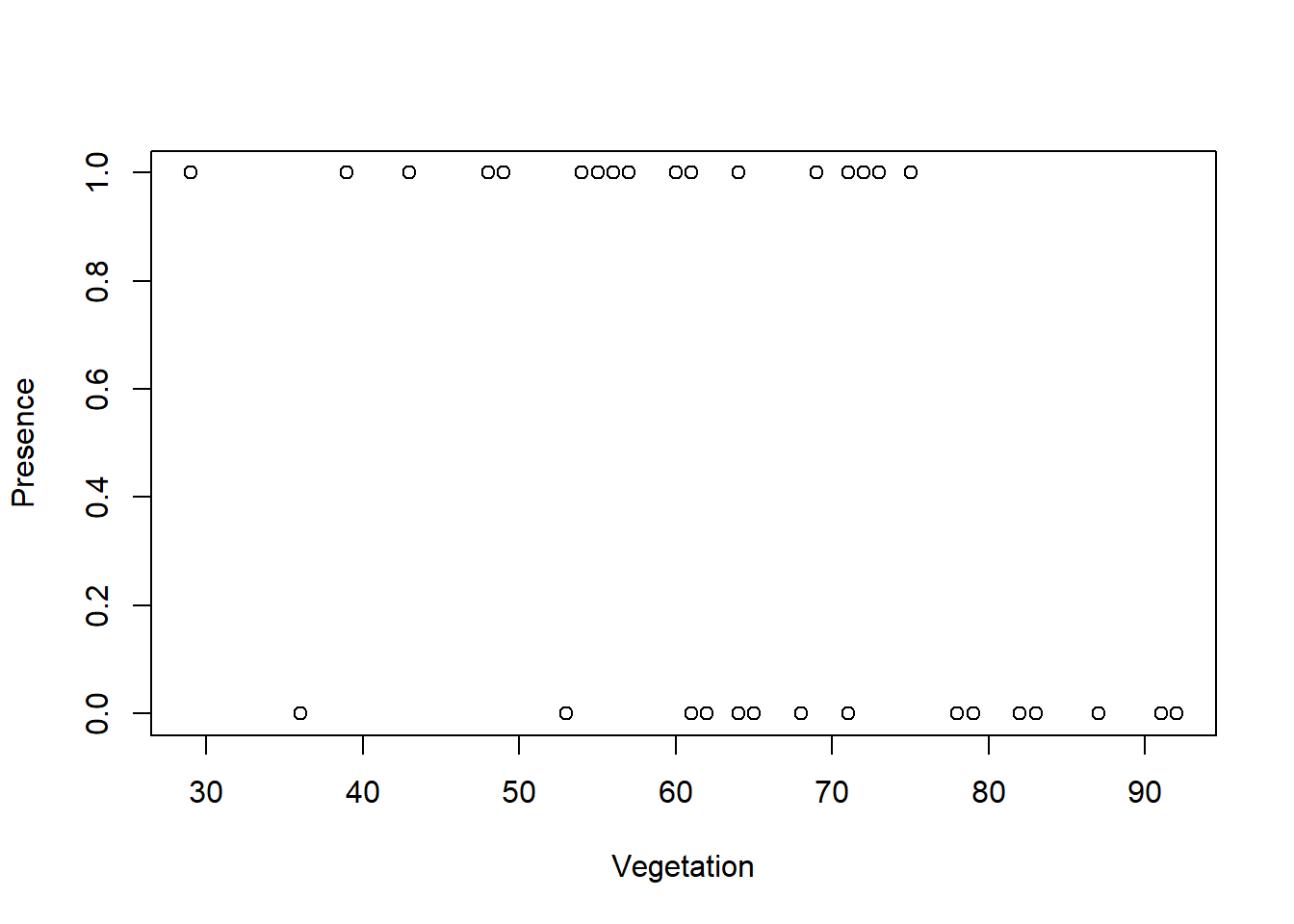

plot(TempMin, Presence)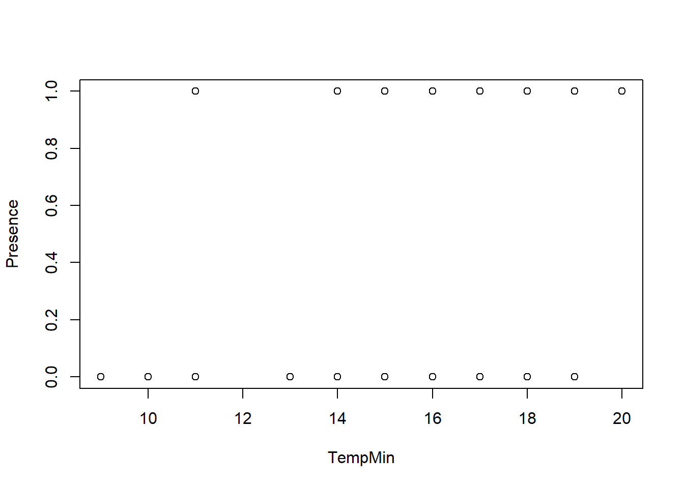

plot(Vegetation,Proportion)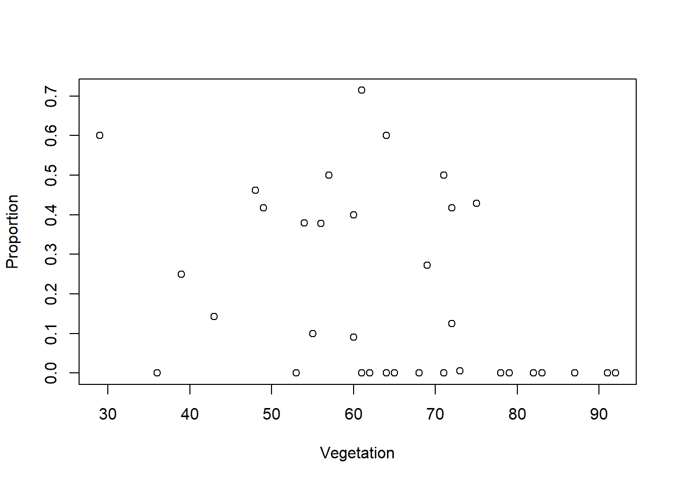

#quick visual check of veg/temp covariation
plot(Vegetation,TempMin)

cor(Vegetation,TempMin) #Pearson correlation coefficient (default)

The count and proportion data are definitely zero-inflated. The highest values that are up for evaluation as outliers are not considerably larger than the others, so I am going to keep them.

I am going to try fitting a binomial glm for the presence/absence data using vegetation cover and minimum temp. I will use the standard link function (logit). Both logit and probit link functions assume that you have approximately an equal number of zeros and ones…and I do!

model1 <- glm(Presence ~ Vegetation + TempMin, family = binomial(link = "logit"),
          data = aedes_dat)

summary(model1)

## 
## Call:
## glm(formula = Presence ~ Vegetation + TempMin, family = binomial(link = "logit"), 
##     data = aedes_dat)
## 
## Deviance Residuals: 
##      Min        1Q    Median        3Q       Max  
## -2.16890  -0.99378  -0.07501   0.99064   1.50534  
## 
## Coefficients:
##             Estimate Std. Error z value Pr(>|z|)  
## (Intercept)  5.39261    4.41440   1.222   0.2219  
## Vegetation  -0.07886    0.03660  -2.155   0.0312 *
## TempMin     -0.01587    0.16782  -0.095   0.9247  
## ---
## Signif. codes:  0 '***' 0.001 '**' 0.01 '*' 0.05 '.' 0.1 ' ' 1
## 
## (Dispersion parameter for binomial family taken to be 1)
## 
##     Null deviance: 52.679  on 37  degrees of freedom
## Residual deviance: 43.933  on 35  degrees of freedom
## AIC: 49.933
## 
## Number of Fisher Scoring iterations: 4

#load car library for easy VIF function
library(car)

## 
## Attaching package: 'car'

## The following object is masked from 'package:dplyr':
## 
##     recode

vif(model1)

## Vegetation    TempMin 
##   1.404985   1.404985

Looks like minimum temperature is not significant when Vegetation is included. I have a p-value < 0.05 for vegetation, so I’ll drop minimum temperature in the model.

model2 <- glm(Presence ~ Vegetation, family = binomial(link = "logit"),
          data = aedes_dat)

summary(model2)

## 
## Call:
## glm(formula = Presence ~ Vegetation, family = binomial(link = "logit"), 
##     data = aedes_dat)
## 
## Deviance Residuals: 
##      Min        1Q    Median        3Q       Max  
## -2.16875  -0.99543  -0.07211   0.98946   1.50902  
## 
## Coefficients:
##             Estimate Std. Error z value Pr(>|z|)  
## (Intercept)  5.02479    2.05386   2.447   0.0144 *
## Vegetation  -0.07703    0.03088  -2.494   0.0126 *
## ---
## Signif. codes:  0 '***' 0.001 '**' 0.01 '*' 0.05 '.' 0.1 ' ' 1
## 
## (Dispersion parameter for binomial family taken to be 1)
## 
##     Null deviance: 52.679  on 37  degrees of freedom
## Residual deviance: 43.942  on 36  degrees of freedom
## AIC: 47.942
## 
## Number of Fisher Scoring iterations: 4

And now I can plot the predicted relationship.

#create new covariate values within observed range for predictions
pred1 <- data.frame(Vegetation = seq(from = 20,
                                    to = 95, by = 5))

Pred <- predict(model2, newdata = pred1, type = "response")

plot(x = Vegetation, y = Presence)
lines(pred1$Vegetation, Pred)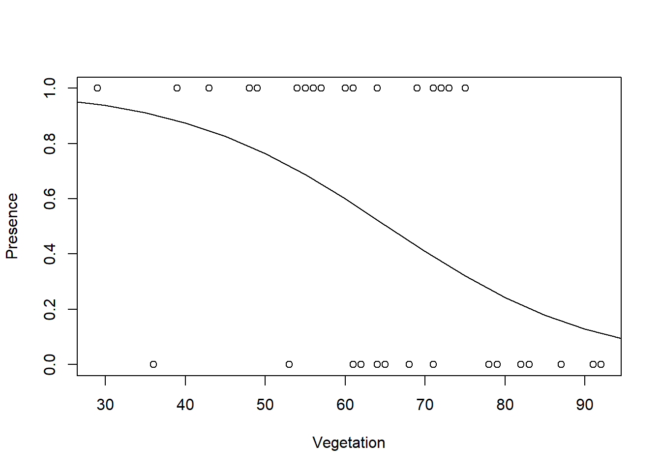

I can use a likelihood ratio test to determine whether the model without minimum temperature is better.

# LR test by dropping each term shows that Vegetation should be retained.
drop1(model1, test = "Chi")

## Single term deletions
## 
## Model:
## Presence ~ Vegetation + TempMin
##            Df Deviance    AIC    LRT Pr(>Chi)  
## <none>          43.933 49.933                  
## Vegetation  1   49.951 53.951 6.0184  0.01416 *
## TempMin     1   43.942 47.942 0.0089  0.92465  
## ---
## Signif. codes:  0 '***' 0.001 '**' 0.01 '*' 0.05 '.' 0.1 ' ' 1

GLM for Proportional Data

I’ll now try using the response variable that is the proportion of Ae. albo out of the whole sample of mosquitoes per site. I’m still going to stick with vegetation cover in a simple regression.

model3 <- glm(Proportion ~ Vegetation, family = binomial,
          data = aedes_dat)

## Warning: non-integer #successes in a binomial glm!

summary(model3)

## 
## Call:
## glm(formula = Proportion ~ Vegetation, family = binomial, data = aedes_dat)
## 
## Deviance Residuals: 
##     Min       1Q   Median       3Q      Max  
## -1.0104  -0.5257  -0.3454   0.3424   1.1523  
## 
## Coefficients:
##             Estimate Std. Error z value Pr(>|z|)
## (Intercept)  1.13912    1.83392   0.621    0.535
## Vegetation  -0.04293    0.02996  -1.433    0.152
## 
## (Dispersion parameter for binomial family taken to be 1)
## 
##     Null deviance: 14.334  on 37  degrees of freedom
## Residual deviance: 12.132  on 36  degrees of freedom
## AIC: 25.903
## 
## Number of Fisher Scoring iterations: 5

Big realization: I probably need to deal with nonlinear responses in my data. I expect that there will be a density of Aedes around species-specific optimal conditions.

Friends, What’s next on this front?

In class we discussed using a quadratic term or GAM.

GLM for count data

I am also interested in general changes in mosquito abundance across the land use gradient. A few studies have shown an increase in overall abundance with forest cover.

Again, I’ll start with data exploration and will take a look at the total mosquito abundance data.

hist(Total, breaks=50, xlab = "Total mosquitoes", main = NULL, freq = FALSE)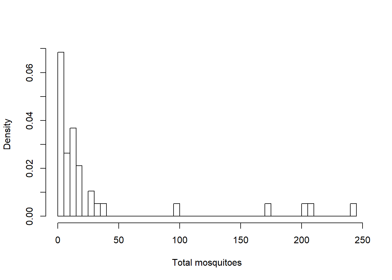

dotchart(Total, xlab = "Total mosquitoes",
         ylab = "Order of data", labels = F)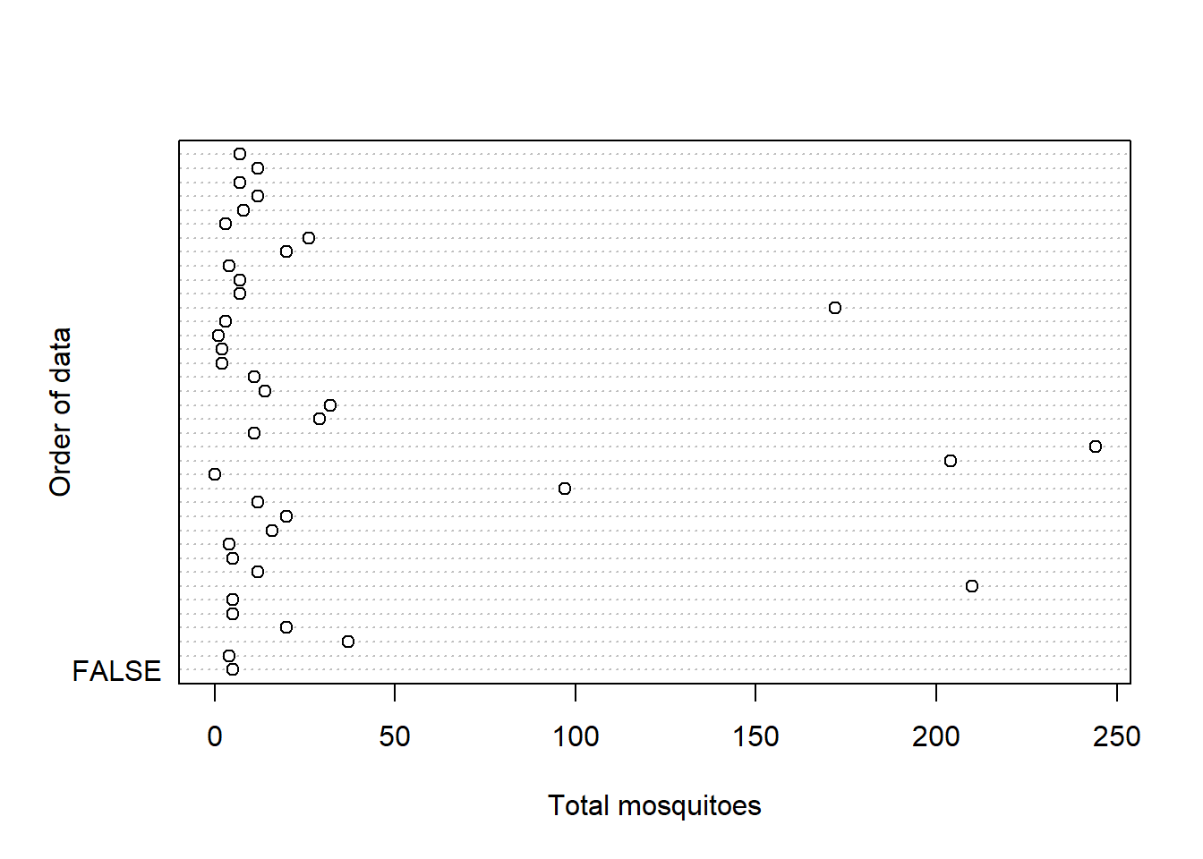

plot(Vegetation,Total)

So I’ve got some really big values at a few sites that had tons of mosquitoes, and they could have a huge influence on my model. What to do?

total.mod1 <- glm(Total ~ Vegetation, family = poisson,
          data = aedes_dat)

summary(total.mod1)

## 
## Call:
## glm(formula = Total ~ Vegetation, family = poisson, data = aedes_dat)
## 
## Deviance Residuals: 
##     Min       1Q   Median       3Q      Max  
## -12.518   -4.969   -2.744    1.616   19.567  
## 
## Coefficients:
##              Estimate Std. Error z value Pr(>|z|)    
## (Intercept) -1.139980   0.173682  -6.564 5.25e-11 ***
## Vegetation   0.065094   0.002209  29.467  < 2e-16 ***
## ---
## Signif. codes:  0 '***' 0.001 '**' 0.01 '*' 0.05 '.' 0.1 ' ' 1
## 
## (Dispersion parameter for poisson family taken to be 1)
## 
##     Null deviance: 2640.9  on 37  degrees of freedom
## Residual deviance: 1642.6  on 36  degrees of freedom
## AIC: 1808.4
## 
## Number of Fisher Scoring iterations: 6

As expected, I have a significant result. I can calculate the explained deviance as the authors do in section 9.5.3, and if this were an accepted result, I would find that vegetation explains 37.8% of the variation in mosquito abundance.

I’ll plot the prediction…

Pred2 <- predict(total.mod1, newdata = pred1, type = "response")

plot(x = Vegetation, y = Total)
lines(pred1$Vegetation, Pred2)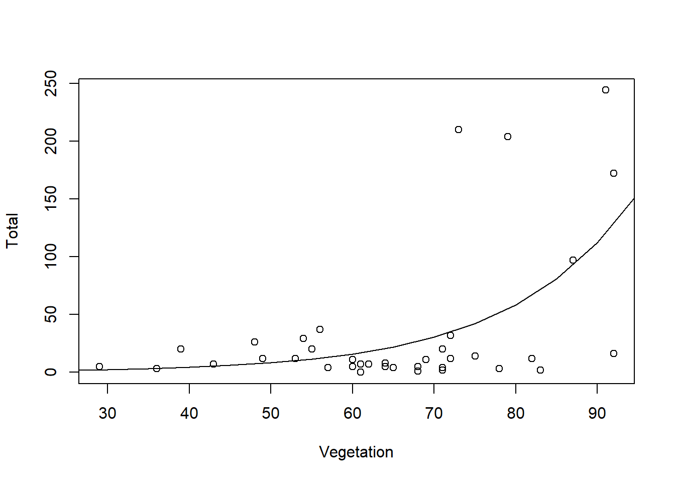

Given that the dispersion parameter is 1, this suggests that I do not have to worry about overdispersion.

Next, validation: We need to take the residuals of choice (e.g. deviance) and plot them against (i) the fitted values, (ii) each explanatory variable in the model, (iii) each explanatory variable not in the model (the ones not used in the model, or the ones dropped during the model selection procedure), (iv) against time, and (v) against spatial coordinates, if relevant. We do not want to see any patterns in these graphs. If we do, then there is something wrong, and we need to work out what it is.

Discussion Questions

Q1: How to validate a binomial GLM model?

Q2: What are potential reasons for choosing between a quasi-Poisson model or negative binomial model to deal with overdispersion?

Q3: I thought these 2 chapters had a lot of information to take in…what are your questions?

After-class follow-up